Chapter 3 Severity of illness and likely outcome from critical illness

At present scoring systems are not sufficiently accurate to make outcome predictions for individual patients.

Clinical assessment of severity of illness is an essential component of medical practice. It influences the need and speed for supportive and specific therapy. Initial acuity may also indicate likely prognosis when other factors such as comorbidity and organisational aspects of critical care delivery are considered. It is intuitive to consider whether patterns and severity of physiological disturbance can predict patient outcome from an episode of critical illness.

Perhaps the earliest reference to grading illness was in an Egyptian papyrus which classified head injury by severity.¹ More recently it has been the constellation of physiological disturbances for specific conditions which popularised an approach which linked physiological disturbance to outcome in the critically ill. Examples include the Ranson score for acute pancreatitis,² the Pugh modification of Child–Turcotte classification for patients undergoing portosystemic shunt surgery and now widely used for classification of end-stage liver disease,³ Parsonnet scores for cardiac surgery⁴ and the Glasgow Coma Score (GCS) for acute head injury.⁵ The earliest attempts to quantify severity of illness in a general critically ill population was by Cullen et al.⁶ who devised a therapeutic intervention score as a surrogate for illness. This was followed in 1981 with the introduction of the Acute Physiology, Age and Chronic Health Evaluation (APACHE) scoring system by Knaus et al.⁷ Since then numerous scoring systems have been designed and tested in populations across the world.

The potential advantages of quantifying critical illness include:

• providing a common language for discussion

• provision of risk-adjusted expected mortality rates facilitating acuity comparisons for clinical trials

• estimates of prognosis

• providing a method by which critical care practice and processes can be examined

The least controversial use for scoring systems has been as a method for comparing patient groups in clinical trials. While this seems to have been widely accepted by the critical care community, there has been less enthusiasm to accept the same systems as comparators for between-unit and even between-country performances, unless of course your performance is good. Most clinicians agree that scoring systems have limited value for individual patient decision pathways, although recently an APACHE II score above 25 under appropriate circumstances has been included in the guidelines for the administration of recombinant human activated protein C for severe sepsis and septic shock. Much of the sceptical views among clinicians are based on studies which show poor prognostic performance from many of the models proposed.⁸^–¹⁴ The fundamental problem for these scores and prognostic models is poor calibration for the cohort of patients studied, often in countries with different health service infrastructures, to where the models were first developed. Other calibration issues arise either because there is poor adherence to the rules for scoring methodology by users, or patient outcomes improve following introduction of new techniques and treatments or models failed to include important prognostic variables. For example it has become clearer that prognosis is as much affected by local organisation, patient pathways, location prior to admission and preadmission state as it is by acute physiological disturbances.^15,¹⁶

Score systems would be better calibrated if developed from a narrow number of countries with similar health services. However this limits their international usefulness for clinical studies. The latter can be improved by score systems developed from a wider international cohort; however when used for an individual country it can be expected to calibrate poorly. Simplified Acute Physiology Score 3 (SAPS 3: developed across the globe) has provided customisation formulae so that the risk-adjusted expected mortality can be related to the geographical location of the unit.¹⁶

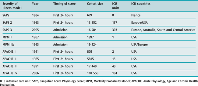
Inevitably, as advances occur, risk-adjusted mortality predictions become outdated with some old models overestimating expected mortality ^14,¹⁷ and others underestimating observed mortality.¹⁸ The designers of the scoring systems have recognised the changing baselines and review the models every few years, Table 3.1 outlines some characteristics of the upgraded systems.

Table 3.1 Revision dates for the most common internationally recognized risk adjusted models for mortality prediction

PHYSIOLOGICAL DISTURBANCE

An insult which potentially interferes with normal organ function is usually followed by increasing compensatory activity in order to retain vital organ activity. Most compensatory mechanisms are mediated through the endocrine and autonomic nervous system directed to maintain effective circulating volume, oxygenation and acid–base homeostasis to ensure normal mitochondrial function and vital organ function. Therefore hyperventilation, tachycardia, vasoconstriction and consequent oliguria – all signs of compensation – are hallmarks of early untreated critical illness. Once overwhelmed, the compensatory mechanisms lead to signs of decompensation such as hypotension, progressive coma, icterus and metabolic acidosis.

Most organs have limited ways in which they manifest their dysfunction in response to a systemic illness, for example the brain responds by becoming confused, developing seizures or progressive coma, while respiratory function is limited to hyperventilation, hypoventilation, wheezing or coughing with commensurate changes in blood gases. Therefore it is not surprising that most systemic pathophysiological processes result in common acute physiological disturbances. Consequently severity of illness can be assessed from a limited number of vital sign and biochemical observations. However it is not so clear what the magnitude of a response should be for a given insult. Therefore severity of illness for most conditions has been traditionally measured by the magnitude of physiological response rather than size of insult. The physiological response is further confounded by:

• Natural variability between patients

• Variable physiological reserve between patients

• Non-linear organ dysfunction in response to an insult, for example both the liver and kidney only manifest biochemical abnormality when a significant proportion of organ mass is malfunctioning

• Poor understanding of relative equivalence of degrees of malfunction between organs, e.g. what degree of jaundice is equivalent to a tachycardia 130 beats/min as an objective measure of severity of illness?

• Impact of organ support on physiological measurements, e.g. inotropes

Some scoring systems such as Mortality Probability Model (MPM II₀) and SAPS 3 estimate severity of illness on or near admission to intensive care in order to avoid the confounding effect of supportive therapy.

PRIMARY PATHOLOGICAL PROCESS

The primary pathology leading to intensive care admission has a significant influence on prognosis. Therefore, for a given degree of acute physiological disturbance, the most serious primary pathologies or underlying conditions are likely to have the worst predicted outcomes. For example, similar degrees of respiratory decompensation in an asthmatic and a patient with haematological malignancy are likely to lead to different outcomes. Furthermore the potential reversibility of a primary pathological process, whether spontaneous or through specific treatment, also greatly influences outcome, e.g. patients with diabetic ketoacidosis can be extremely unwell but insulin and volume therapy can rapidly reverse the physiological disturbance.

Both APACHE and the most recent SAPS systems include diagnostic categories with different weightings which improve the precision of estimated risk of hospital death calculations.

PHYSIOLOGICAL RESERVE, AGE AND COMORBIDITY

Physiological reserve is a surrogate term which broadly combines age and health status prior to critical illness. Age may be associated with diminishing physiological capacity but not in a predictable fashion.

• Chronological age alone is not a very strong influence on outcome.

• Biological age is a vague term usually used to imply physiological reserve below that expected for a patient’s chronological age. Biological age greater than chronological age is common in patients who smoke heavily, abuse alcohol or who have insidious systemic diseases such as diabetes and hypertension; these patients typically have reduced reserve of one or more organs.

Chronic health states such as immunosuppression, cirrhosis, cancer and haematological malignancies all result in significant diminution of physiological reserve and may have an overwhelming influence on outcome. These conditions are commonly included in any assessment of critical illness.

SOURCE OF ADMISSION AND MODE OF PRESENTATION

Patients arriving in intensive care either come as an emergency or for a variety of reasons come following elective surgery. There are a very small number of patients who come to intensive care for elective medical reasons. By its very nature emergency admission implies that patients are likely to be unstable and that the acute physiological disturbances are in the process of being managed. Most scoring systems quantifying risk of death include an adjustment for emergency admission. It has become widely recognised that the source of admission also influences the likely outcome. This might in part be because it increases the likelihood of patients having resistant organisms, such as those admitted from a health care environment.

ORGAN SUPPORT PRIOR TO ADMISSION

Many patients may arrive in ICU already ventilated, and receiving inotropes. Assessment of severity of illness at this stage when some physiological abnormalities have been corrected would make a physiologically based assessment underscore. Therefore either the assessment has to be adjusted to a time when no organ support was provided or some allowance has to be made for the support in the assessment. The approach to this has been varied; for example, SAPS 3 makes an adjustment for patients on inotropes, whereas MPM II allows measurements for the hour on either side of admission to be included.

UNIT ORGANISATION AND PROCESSES

Soon after the introduction of APACHE II it was recognised that units with effective teams, nursing and medical leadership, good communications and run by dedicated intensive care specialists potentially had better outcomes than those without such characteristics.¹⁹^–²¹

OTHER FACTORS

Some factors have not been included in risk-adjusted models for prediction of mortality; these include socioeconomic and genetic variables. However SAPS 3 has included a customisation adjustment to calibrate their model for patients in different parts of the world, possibly taking account of local factors and health care systems.

RISK-ADJUSTED EXPECTED OUTCOME AND ITS MEASUREMENT

Physiological disturbance, physiological reserve, pathological process and mode of presentation can be related to expected outcome by statistical methods. Common outcome measures for clinical trials are ICU mortality, or mortality at 28 days; however most models used for risk-adjusted mortality prediction are based on hospital mortality. Patient morbidity might also be considered nearly as important an endpoint as mortality, since many patients survive with serious functional impairment.^22,²³ For socioeconomic reasons there would be a strong argument to consider 1-year survival and time to return to normal function or work as endpoints.^24,²⁵ These latter measures however have been more closely related to chronic health status.

Hospital mortality is the most common outcome measure because it is frequent enough to act as a discriminator and is easy to define and document.

PRINCIPLES OF SCORING SYSTEM DESIGN

CHOICE OF INDEPENDENT PHYSIOLOGICAL VARIABLES AND THEIR TIMING

The designers of the original APACHE and SAPS systems chose variables which they felt would represent measures of acute illness. The chosen variables were based on expert opinion weighted equally on an arbitrary increasing linear scale, with the highest value given to the worst physiological value deviating from normal.^26,²⁷ Premorbid conditions, age, emergency status and diagnostic details were also included in these early models and from these parameters a score and risk of hospital death probability could be calculated. Later upgrades to these systems, SAPS 2, APACHE III and the MPM,²⁸ used logistic regression analysis to determine the variables which should be included to explain the observed hospital mortality. Variables were no longer given equal importance but different weightings and a logistic regression equation were used to calculate a probability of hospital death. The more recent upgrades, APACHE IV and SAPS 3, have continued to use logistic regression techniques to identify variables that have an impact on hospital outcome.

The extent of physiological disturbance changes during critical illness. Scoring systems therefore needed to predetermine when the disturbance best reflected the severity of illness which additionally facilitated discrimination between likely survivors and non-survivors. Most systems are based on the worst physiological derangement for each parameter within the first 24 hours of ICU admission. However some systems, such as MPM II₀, are based on values obtained 1 hour either side of admission; this is designed to avoid the bias that treatment might introduce on acute physiology values.²⁹

DEVELOPING A SCORING METHODOLOGY AND ITS VALIDATION

All the scoring systems have been based on a large database of critically ill patients, usually derived from at least one country and from several ICUs (Table 3.2). Typically, in the more recent upgrades of the common scoring systems, part of the database is used to develop a logistic regression equation with a dichotomous outcome – survival or death, while the rest of the database is used to test out the performance of the derived equation. The equation includes those variables which are statistically related to outcome. Each of these variables is given a weight within the equation. The regression equation can be tested, either against patients in the developmental dataset using special statistical techniques such as ‘jack-knifing’ and ‘boot-strapping’ or against a new set of patients – the validation dataset – who were in the original database but not in the developmental dataset. The aim of validation is to demonstrate that the derived model from the database can be used not only to measure severity of illness but also to provide hospital outcome predictions.

Table 3.2 Ability of scores to discriminate correctly between survivors and non-survivors when tested on similar casemixes. A value of 1 represents perfect prediction

Score	Area under ROC curve
APACHE II	0.85
APACHE III	0.90
SAPS 2	0.86
MPM II₀	0.82
MPM II₂₄	0.84
SAPS 3	0.84
APACHE IV	0.88

ROC, receiver operating characteristic; APACHE, Acute Physiology, Age and Chronic Health Evaluation; SAPS, Simplified Acute Physiology Score; MPM, Mortality Probability Model.

Once a satisfactory equation has been developed it can be used to calculate a probability of death for an individual patient. Similarly an overall probability of death can be calculated for a group of patients; however, this methodology can not indicate which of the patients in the cohort is going to die. These models are not powerful enough to provide sufficiently accurate discrimination.

In a perfect model the aim would be that:

• Overall predicted and observed outcomes should be the same.

• Individual patients observed to die or survive have been predicted.

The performance of a mortality prediction model used on a cohort of patients other than the developmental set is usually judged by two functions: first, its ability to predict which patients will survive and which will die (discrimination) and second, how well a model correctly predicts the overall observed mortality (calibration). The appendix shows some commonly calculated measures for a scoring system.

DISCRIMINATION

The discriminating power of a model can be determined by defining a series of threshold probabilities of death such as 50, 70, 80% above which a patient is expected to die if their calculated risk of death exceeds these threshold values and then comparing the expected number of deaths with what was observed in those patients at the various probability cut-off points. For example, the APACHE II system revealed a misclassification rate (patients predicted to die who survived and those predicted to survive who died) of 14.4, 15.2, 16.7 and 18.5% at 50, 70, 80 and 90% cut off points above which all patients with such predicted risks were expected to die. These figures indicate that the model predicted survivors and non-survivors best i.e., discriminated likely survivors from non-survivors when it was assumed that any patient with a risk of death greater than 50% would be a non-survivor.

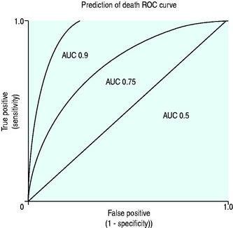
A conventional approach to displaying discriminating ability is to plot sensitivity, true positive predictions on the y-axis against false-positive predictions (1 – specificity) on the x-axis for several predicted mortality cut-off points, and producing a receiver operator characteristic curve (ROC) (Figure 3.1).

Figure 3.1 A receiver operator curve (ROC) plots true-positive against false-positive rates for a series of cut-off points for risk of death. For example, a risk of death cut-off point of 10% would predict that all patients with a risk greater than 10% will die and all those below will survive. This would be compared with the observed rates in those patients. The prediction would be expected to be frequently wrong and would reflect itself in the calculation of true-positive and false-positive rates. These calculations would represent one point on the ROC curve. The exercise is repeated at different cut-off points, such as 15, 20, 25, 30, from which a curve can be constructed. The resulting area under the curve (AUC) reflects the ability of the model to predict survival correctly. This is a measure of discriminatory power. The best models have values greater than 0.85.

The ROC area under the curve (AUC) summarises the paired true-positive and false-positive rates at different cut-off points (Figure 3.1) and provides a curve which defines the overall discriminating ability of the model. A perfect model would show no false positives and would therefore follow the y-axis and has an area of 1, a model which is non-discriminating would have an AUC 0.5, whereas models which are considered good would have AUC greater than 0.8. The AUC can therefore be used for comparing discriminating ability of severity of illness predictor models.